Clustering for Threat Detection: Machine Learning in Cybersecurity

Author Credits: Alvin Wen, Software Architect, and Craig Chamberlain, Director of Algorithmic Threat Detection

Many modern standards, practices, and frameworks, including the MITRE ATT&CK matrix, emphasize the importance of discerning the unusual from the malicious in modern event logs and detections, which often contain many shades of gray between the interesting and the confirmed true positive threat detection. 

The MITRE ATT&CK matrix makes extensive recommendations to “baseline” normal activity. It contains at least 154 references to baselining normal activity, or monitoring for anomalous activity, as shown below. This guidance is necessary in order to discern the few malicious events from the great mass of benign events typically present in system logs. But MITRE ATT&CK does not discuss practical methods of undertaking baselining or anomaly detection at scale.

So what are we to do? This is where we need to add machine learning tooling to our threat hunting and detection practices. There are a number of powerful tools we can bring to bear, not to replace conventional detection, rather to supplement and assist it.

Table 1

This blog post discusses our research and development on clustering of compute workloads. Workloads can be 1) containers, in container fleets or 2) virtual servers, in cloud server fleets. Clustering can be used to find both “drift” detection and threat detection. Drift detection essentially means that a workload has configuration or software attributes that diverge from the population it belongs to. Drift detections can range the gamut of risks from poor security “hygiene” in the form of unpatched software or can be something more serious such as a persistence mechanism, like a backdoor, or even a supply chain poisoning attack. 

Threat detection, using clustering, involves finding unusual behaviors in masses of system log event streams such as process and network events. Such unusual behaviors can produce findings of a wide variety of tactics including persistence, lateral movement, C2, and exfiltration.

Machine learning

Machine learning, in addition to uncovering threat activity that may be resistant to conventional detection, as with LOLbins, for example, and credentialed access, where the difference between benign and malicious is the smallest matter of nuance, in shades of gray too fine to be expressed in a query based rule language. 

Machine learning, at the same time, can often help us find what’s coming next, even when we don’t yet know what “next” is, and cannot write rules for it. Machine learning, unlike conventional rule-based detection, is not dependent on prior knowledge of the threat activity we are looking for, and so can find emerging threats even before new threat intelligence is available. 

Several types of machine learning can be brought to bear. There are an increasing number of trained models for classification and detection of malicious phenomena such as malware execution, malicious URLs, phishing and DGA (domain generation algorithms.) Classification models generally need extensive training on labeled data sets. For unlabeled data sets, as we typically have with the types of log streams utilized in security detection and threat hunting practices, we can employ other approaches including anomaly detection and clustering.

Infrastructure-as-Code

In threat hunting practices, sometimes it is immediately clear that something just discovered in the data is going to rapidly become a critical incident response case replete with war rooms, ongoing conferences, and regular reports to leadership. Certain security events like VPN connections from Eastern Europe, password dumping artifacts on domain controllers, C2 (command and control) activity with a destination in Moscow, and perhaps cloud virtual machine activity sourcing from Beijing, might go directly to incident response without question. More often, we face more shades of gray, as first results are not clear enough to initiate such action. 

The activity in question, while unusual, might actually be benign activity coming from an authorized user or process. For example, one day I was conferring with an esteemed colleague from an external organization as we sifted a great mass of event log data, and he remarked, “is ClamAV (a FOSS antivirus tool) supposed to be talking to something in Germany?” The answer, of course, was, “I have no way of knowing that, at least not immediately.” 

In order to answer this question, quite a lot of prior knowledge would have to be in place. What is the baseline network behavior for this particular software tool? Does it call the same destination, or does it call a CDN (content distribution network)? What are the AS (autonomous system) names of the normal destinations, and what are their geolocations? What kind of requests does it make, and how often? Does it simply make periodic requests for new data and/or updates, or does it usually send telemetry? While it might be possible to construct such a baseline for one or two software tools, or maybe a dozen, the task becomes Sisyphean at scale. Modern distributed systems contain hundreds of software products and platforms, each of which may change its behavior with every new release.

The rise of “infrastructure as code” is creating distributed systems that change and evolve too rapidly for human analysts to baseline and profile expected behavior.

Modern information systems are highly distributed and operate at great scale and complexity. Cloud-based systems often do not have notions of fixed networks, hostnames, IP addresses, or physical locations that can be enumerated and turned into lists. The rise of “infrastructure as code” is creating distributed systems that change and evolve too rapidly for human analysts to baseline and profile expected behavior. In the post-COVID era of remote work, users are also often widely distributed, breaking old paradigms revolving around office networks and choke points like VPNs and firewalls.

One example is the increasing ambiguity of network behavior and the diverse nature of network socket events. Years ago, a popular hunting technique involved looking for server instances initiating outbound connect events. Servers, the theory went, should be accepting connections from clients, and producing accept or listen events, not spontaneously initiating connections of their own. The modern reality today is that most popular software frameworks expect the Internet to be “always on” so they can “phone home” to make network requests for updates, schemas, data, or other artifacts. While “home” may be a parent organization, the destination hostname and IP address is likely to be part of a medium or large sized global content distribution network, not a short list of things that can be enumerated and turned into a list. 

Modern operating systems increasingly send telemetry, in addition to checking for updates, that may resemble C2 (command and control) activity in packet size and frequency. LoLbins, or living off the land binaries, and their equivalents for the Linux and MacOS platforms, create innumerable dual-use programs and behaviors, of which an infinitesimally small number are actually suspicious or malicious in nature. 

All of these factors complicate the work of threat hunting practices by exponentially growing the process, network, dns, file, and other behaviors of distributed systems, creating an increasingly vast forest of benign behavior, with many normal outliers of every possible description.

ML Clustering

In the world of cybersecurity, threat detection can resemble a search for needles in haystacks. We are looking for unusual processes, abnormal network activity, or data access patterns that fall outside of the norm. While we may have access to tools that allow us to efficiently search through huge volumes of logs, many events or configurations that correlate with threats in certain contexts may be completely benign in others.

This is where machine learning (ML) clustering can come into play. By analyzing patterns of behaviors associated with entities and grouping entities with similar behaviors together, clustering helps us find outlying behaviors that may not be distinctive when considered as part of a whole but which are unusual specifically when examined in the context of similarly behaving entities. (For the purpose of this blog, an "entity" could be a physical or virtual endpoint, a container image, or a user or role.)

Some applications of clustering for threat detection include:

• Detecting irregular endpoint configuration.
  
  
• Detecting unusual user, host or container behaviors, as compared with similar hosts or containers.
  
  
• Detecting changes in activity patterns of users, hosts or containers over time.

We will discuss many of these applications below.

Clustering concepts

Distance

In order to apply clustering to a set of entities, we first define what it means for two entities to be similar to each other in behavior or configuration. It's helpful to think of similar entities as being close to each other in location, as in Figure 1 below, where entities have been grouped into four clusters denoted by color.

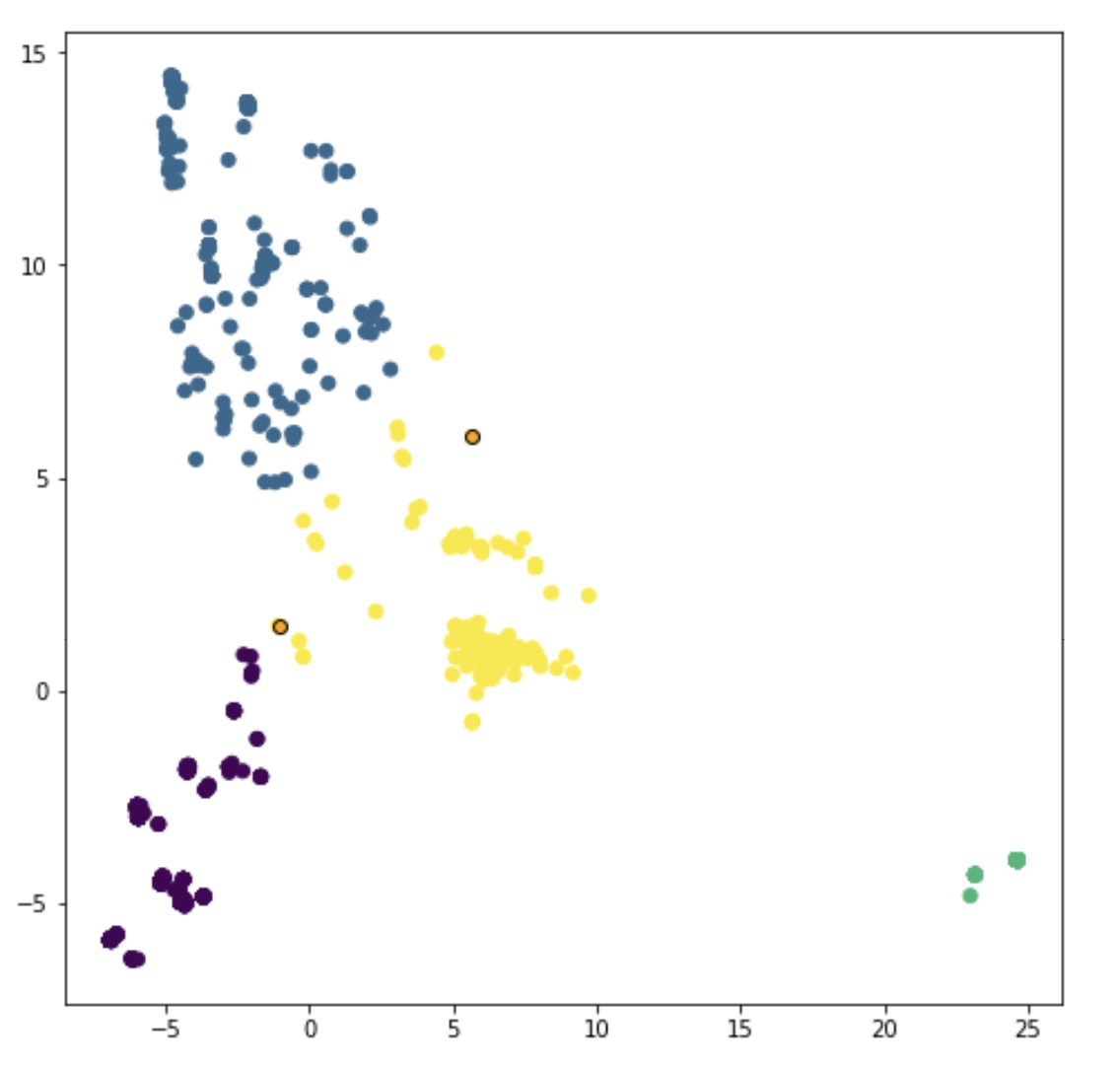Figure 1 – A set of entities grouped into four clusters based on their activity logs, with two outliers identified (in orange)

So, for any given clustering exercise we will compute the distance between entities in a way that corresponds to their similarity in the aspects that we wish to characterize. This is where the ML concept of "feature engineering" comes into play. We will associate features with each entity to characterize its position relative to other entities. Entities with similar features are mathematically near each other, while those with differing features are farther apart. With appropriate system logs, we can use features like the following when grouping entities into clusters for the purpose of threat detection:

• Processes launched
• Network activity, such as connections initiated or accepted, port numbers, and/or remote IP addresses
• System calls
• File system activity
• Packages or programs installed on a host

Once we have a collection of numeric feature values describing each entity, we can compute a mathematical distance between any two entities and use these distances to group similar entities together into clusters. We can also identify outlier patterns of behaviors that are abnormal in the context of an entity's cluster.

Normalization

For best clustering performance when combining features of different types, we will need to normalize  our feature values so they work well together when combined to produce distance values. Essentially, this means that each feature value should be normalized to the same scale, typically in the range from 0.0 to 1.0.

Practically, this may mean transforming absolute counts into fractions--instead of counting the number of times curl  was launched in an hour, we might divide that hourly count by the total counts of all of the processes launched by that entity in that hour. We would do the same with the counts of each of the executables that we wish to include. (Note that this particular approach tends to blur differences between more active and less active entities, putting hosts of different hardware types on equal footing as an example. Leaving the feature values as absolute counts would preserve differences in load, but would also make it different to sensibly combine such features with other features in the same model.)

Categorical features like packages installed can be represented as binary values, with a value of 1.0 meaning that a package is present and 0.0 meaning that it is absent.

Dimension reduction

Some features such as executable names, remote IP addresses, and packages installed may have a large number of distinct values. In ML parlance, these are called high-dimensional features.

In order to make the clustering process more efficient in the presence of high-dimensional features, we can apply techniques for dimension reduction. The most common method of dimension reduction is called PCA, or Principal Component Analysis. PCA creates an optimal mapping of features onto a much smaller number of dimensions (we can specify the number). We can then use these lower-dimensional features to efficiently cluster our entities, typically with very little loss of fidelity.

A side benefit of PCA is that it computes a measure of the relative importance of each feature, as measured by "explained variance." This tells us which features most effectively capture the differences between entities, and can help us prune features and tune PCA dimensions for efficiency.

Note however, that the PCA process itself can be quite time-consuming. In fact, in our own experience the majority of time taken for clustering is spent during PCA.

Approaches to clustering

There are many ML approaches to clustering, a few of which include:

• Centroid-based clustering, e.g., k-means. K-means attempts to group entities into a specified number of clusters so that the variance within each cluster is minimized. While finding the optimal k-means solution is theoretically very hard, in practice approximations like Lloyd's algorithm and k-means++ quickly produce very good solutions. Using the k-means approach, outliers are the entities that lie furthest from the centers of their clusters. The clusters in Figure 1, above, were identified using k-means clustering.
• Hierarchical clustering  groups entities together with their nearest neighbors until reaching the specified number of clusters. The bottom-up approach to hierarchical clustering is called agglomerative clustering . Interestingly, while k-means takes longer for larger numbers of clusters, agglomerative clustering has the opposite behavior--it is faster for larger numbers of clusters.
  
• The Local Outlier Factor (LOF) algorithm specifically tries to find outliers, rather than the clusters themselves. LOF computes a measure of the density of entities close to any given entity, and identifies as outliers those entities with the lowest surrounding density.

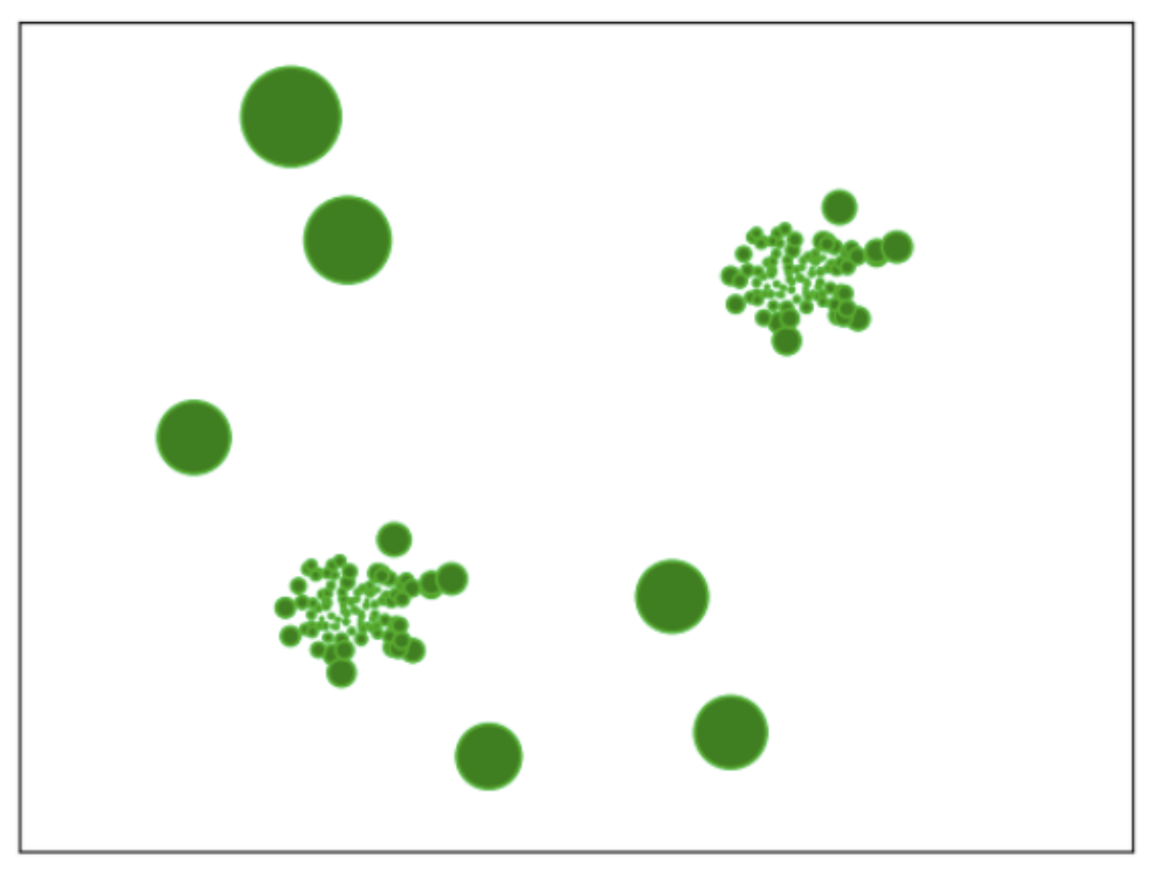Figure 2 – The Local Outlier Factor algorithm applied to a set of entities. The size of each circle represents its outlier score

For the applications discussed below, we confine our discussion to centroid-based clustering, specifically k-means. 

What is an outlier?

Once we have grouped our entities into clusters, we are able to identify outliers, or entities whose behaviors or configurations are anomalous with respect to their clusters. One way we can identify outliers is from a relative perspective: Given a cluster, show me the top n or top n% of entities furthest from its center. We can alternatively identify outliers from a statistical perspective: Show me all entities that lie outside of the 95th percentile of their clusters' distributions.

We can also examine clusters that are unusually small. A cluster containing only one entity is an outlier by definition, and clusters with only a few entities should certainly be scrutinized as well.

Using external labels to evaluate clustering

In some cases, we may be able to use labels for our entities that are not part of our features to help understand whether the makeup of our ML clusters aligns with expectations. Examples of this sort of external label can include:

• Container image names
• Common hostname prefixes
  
• Tags manually applied to entities, such as webserver, jenkins, or developer

Given our ML-computed clusters and external labels for entities, how can we evaluate how well the two align? Here are two approaches:

• The Rand score examines every unique pair of entities in our cluster--if there are n entities then there are n(n-1)/2 unique pairs--and computes the ratio of pairs with matching external labels, divided by the total number of pairs. A Rand score of 1.0 indicates perfect alignment between clusters and labels, while a Rand score of 0 would signal a complete mismatch.
  
  
• The Mutual Information score is a measure of how reliably we can predict the external label given our cluster assignment, and vice versa. Like the Rand score, the worst possible Mutual Information score is 0, but unlike the Rand score, there is no numeric upper bound on the best possible Mutual Information score. 

Applications of clustering for threat detection

Detecting irregular endpoint configuration

With periodic snapshots of endpoint configuration details, we can use clustering to group endpoints with similar configurations, and identify outlier endpoints that may have irregular configurations. For example, we can cluster Linux endpoints by the packages that they have installed, and understand which endpoints have expected packages missing, or non-standard packages installed as compared with similarly configured endpoints.

Visualizing configuration differences

While PCA helps us to cluster entities more efficiently, it also combines features in ways that can make the results difficult to explain. To remedy this problem, once we have used clustering to identify outlier entities with irregular configurations, we can use the entities' original features values to visualize and explain their configuration differences.

Assuming that we use package names as features, with a value of 1 indicating that a package is present and 0 indicating that a package is absent, then we can describe an outlier host as follows:

1. Compute the mean value of all features across all of the hosts in the outlier's cluster. The value of each feature (package name) will contain the fraction of hosts in the cluster that has the package installed. A value of 1.0 would indicate that every host has a package installed, while a value of 0.5 means that a package is installed on exactly half of the hosts in a cluster. This collection of features describes the configuration of the conceptual center of the cluster.

2. For each package installed on the outlier host, subtract the feature value of the cluster center from the feature value of the outlier, and display the results with the largest values (whether positive or negative). A large positive value indicates that the outlier has an unusual package installed, while a large negative value indicates that the outlier is missing a commonly installed package.

Here is an example of a package outlier we found:

These results indicate that the outlier is the only host in its cluster with an end of life version of the Lua package installed which dates to 2015. This version’s last release was 5.3.6 in September 2020 and there are several CVEs in the version found here. While this could well simply be an older workload instance that has been forgotten over time, it has some risk attached, and it is worth looking at because Lua is occasionally used by malware implementations. 

In addition, we can also find cases of packages that are normally pervasive across a fleet of containers or virtual servers, but are unusually absent on certain workload instances. In these examples, a workload was missing a couple of Linux compilers that were pervasive across the fleet:

If we had found missing security instrumentation or tooling, we might ask why it was missing from one or two workload instances and how that occurred. In this case, we probably find ourselves asking a bigger question: why are compilers installed on most of the production fleet? Removing compilers from production workloads, particularly Internet-facing server instances, is a prudent hardening practice. The presence of a local compiler can be convenient for threat actors as discussed in technique T1027.004, Obfuscated Files or Information: Compile After Delivery.

Detecting unusual entity behaviors

Features such as processes launched, network port activity, and so forth, can be used, either separately or in combination, to cluster entities like hosts, containers, or users according to their historic activity patterns. As an example, the name of a feature might be the executable name, and the value might be the number of times the executable was launched by a host or user in the past day.

When used separately, you might not need to normalize feature values like these. This would tend to preserve the differences between lightly- and heavily-loaded machines and also makes the results easier to interpret. On the flip side, having non-normalized features makes it difficult to use a feature in combination with other features, which might have much smaller or larger numeric values.

Visualizing behavior differences

As above, to visualize the behavior of an outlier in a cluster, we first compute the mean value of each feature value across all of the members of a cluster, and then compute the difference between each of the feature values of the outlier and that of the cluster center. When interpreting unusual entity behaviors from a threat perspective, the presence of an unusual behavior is generally more interesting than the absence of an expected behavior, so in contrast to the configuration example above, we can usually disregard large negative values when visualizing behavioral differences.

In the example below, we have an outlier behavior where a java worker process is making connections to an unusual network on an unusual port. This is useful for threat hunting in scenarios like log4j where java web applications make unusual web requests and connections during exploitation and execution. In another case, we found anomalous network behavior on a github runner - part of the build system for a software release train. Given the difficulty of detecting supply chain compromise - where we may be looking for one malicious file among millions -detecting outlier behaviors on supply chain build system workers is a good and practical option today. When a supply chain asset is involved, we can raise the priority of the outlier detection by enriching the data with information that the workload involved is part of a software build system.

Figure 3 - Outlier network behavior by a java worker

In this example, we found tor activity on a virtual server. Tor (the onion router) is a dual-use framework for anonymous Internet communication. While it is used for legitimate research, in many cases, its presence in a production server fleet is uncommon and unexpected most of the time. Unless the workload in question is engaged in security research, the presence of tor activity would be a critical incident in most cases.

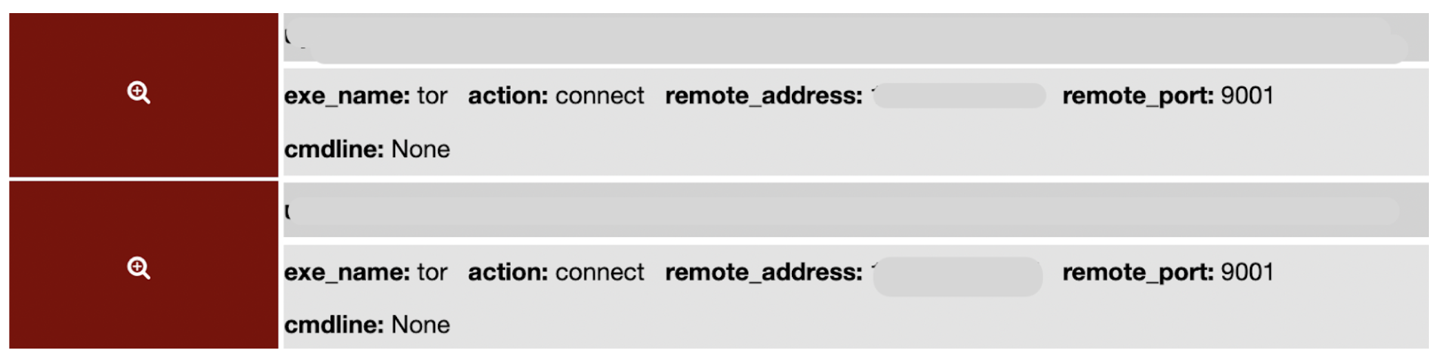Figure 4 - Tor activity on a workload

Understanding behavioral drift

You may want to understand whether or not your clusters are stable over time. Our confidence in outlier detection would certainly be diminished if it turned out that entities were being assigned to different clusters each day. In this section we'll discuss approaches to understanding and measuring clustering stability.

Understanding cluster stability over time

Let's suppose that we grouped hosts into clusters yesterday, based on some behavioral features, and we want to understand how similar or different those clusters are today. We can compute a measure of the stability of our clusters like so:

1. We'll consider only the entities for which we have data both yesterday and today. (If there aren't many entities that are present on both days then we know immediately that we will not have stable clusters day-over-day.)

2. We run k-means to cluster those entities based on yesterday's logs and run it again with the same number of clusters (k) to group them based on today's logs. Now we can measure the similarity between yesterday's and today's clusters.

The assignment problem

For each of yesterday's clusters, we need to figure out which cluster it best corresponds to today. More precisely, we want to match yesterday's clusters with today's in a way that minimizes the total distance that all of the centers move. In Computer Science, this is an example of the Assignment Problem.

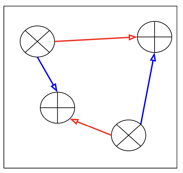Figure 5 – The Assignment Problem: Which arrows (red or blue) minimize the overall distance moved by the cluster centers?

The optimal assignments can be determined using a technique know as the Hungarian Algorithm, which is theoretically very expensive but quite fast in practice.

Assessing the Quality of the Assignments

Now that we have matched each of yesterday's clusters to a cluster today, how can we assess the stability of the assignments?

1. We can compute the Jaccard index, or similarity coefficient, of each of yesterday's clusters with its match today. The Jaccard index for a given pair of clusters is the size of its intersection divided by the size of its union. A perfect match will have a Jaccard index of 1.0. Note that in this situation, very low Jaccard indexes for multiple clusters may be a sign of incorrect assignments rather than unstable clusters.

2. If we have external labels for the entities, we can compare the Rand or Mutual Information scores of each cluster yesterday as compared to today.

Be aware that day-to-day variability in usage patterns can have a significant effect on clustering results. For example, the behavior of some entities on weekends may be quite different from their behavior on weekdays.

Acknowledgements

Special thanks to Thy Dinh Nguyen of Northeastern University for his assistance in the creation of this blog.